目的:介绍用python的MNE预处理EEG数据,并绘制ERSP
EEG analysis with MNE-Python
This tutorial covers the basic EEG pipeline for event-related analysis: loading data, preprocessing, epoching, averaging, plotting, time-frequency analysis, and estimating cortical activity from sensor data.
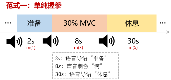
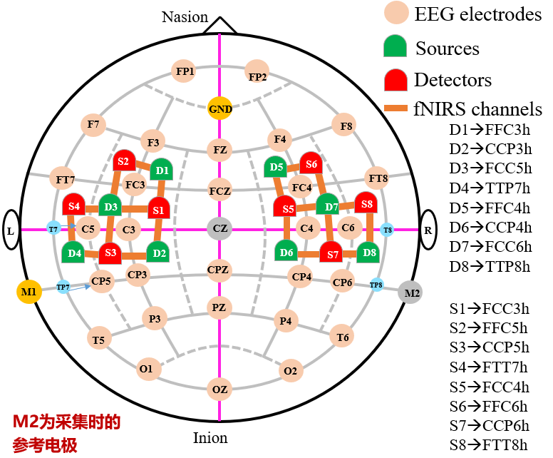
一、实验范式
二、预处理
1. 加载package
1 | import os |
2. 加载数据
1 | path = '.\\EEG\\set\\' |
3. 设置眼电、心电、去除不要的channel
这里根据你自己的电极来设定
1 | pd.DataFrame(raw.ch_names) # 查看通道名称 |
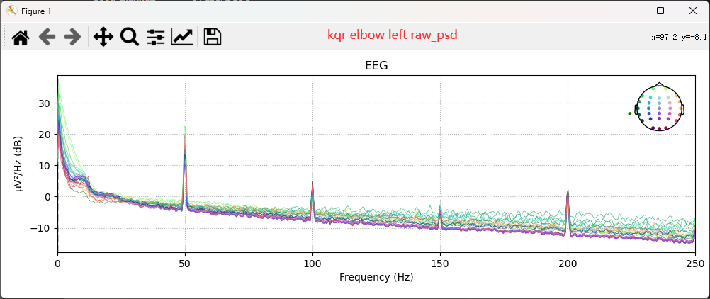
4. 查看raw数据波形,关注信噪比,该数据是否可用【坏导插值】
4.0 查看raw波形,绘制psd
1 | raw.plot(start=10, duration=1) # 从10s开始,窗口显示时长1s |
4.1 挑选坏导
把认为是坏导的,鼠标左键点击一下变灰即可
1 | raw.plot(start=10, duration=1, title='请选择需要插值的坏导') # 从20s开始,窗口显示时长1s |
4.2 插值坏导
1 | raw.load_data() # 默认情况下,MNE不会将数据加载到主内存以节约资源。插值需要加载原始数据。在构造函数或raw.load_data()中使用preload=True(或字符串)。 |
5. 带通滤波:2 ~ 40 *
1 | raw_filter = raw.copy() |
6. 重参考 *
1 | raw_ref = raw_filter.copy() |
6.1 双侧乳突参考
因为我在采集数据时,用的参考电极是M2,这里再次选择双侧乳突参考的原理参考这篇文章
1 | ''' 1. 添加 M2,值为0 ''' |
6.2 平均参考
平均参考的话,一般放到ICA之后
1 | raw_ref.set_eeg_reference(ref_channels='average') |
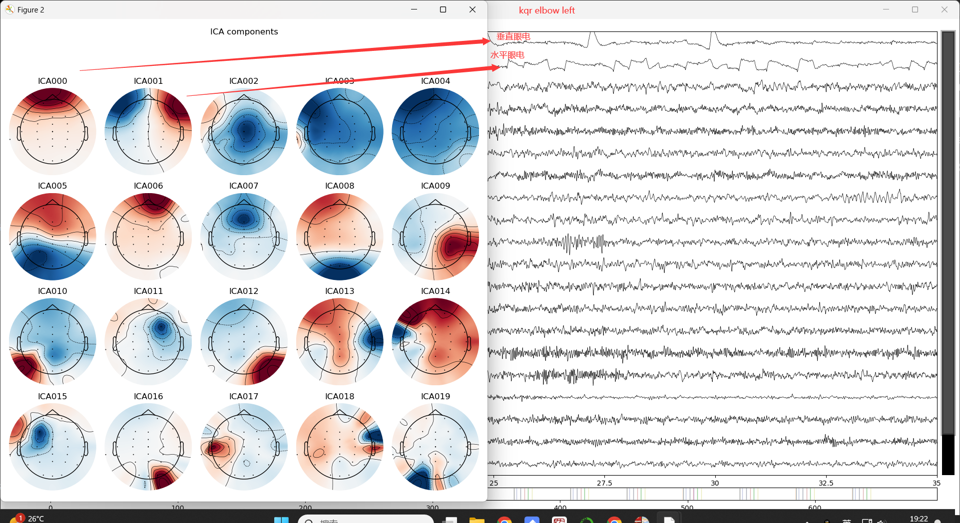
7. ICA去眼电 *
7.1 选取需要去除的ICA成分
1 | ''' 1. ICA,独立成分分析去除眼电和心电伪迹''' |
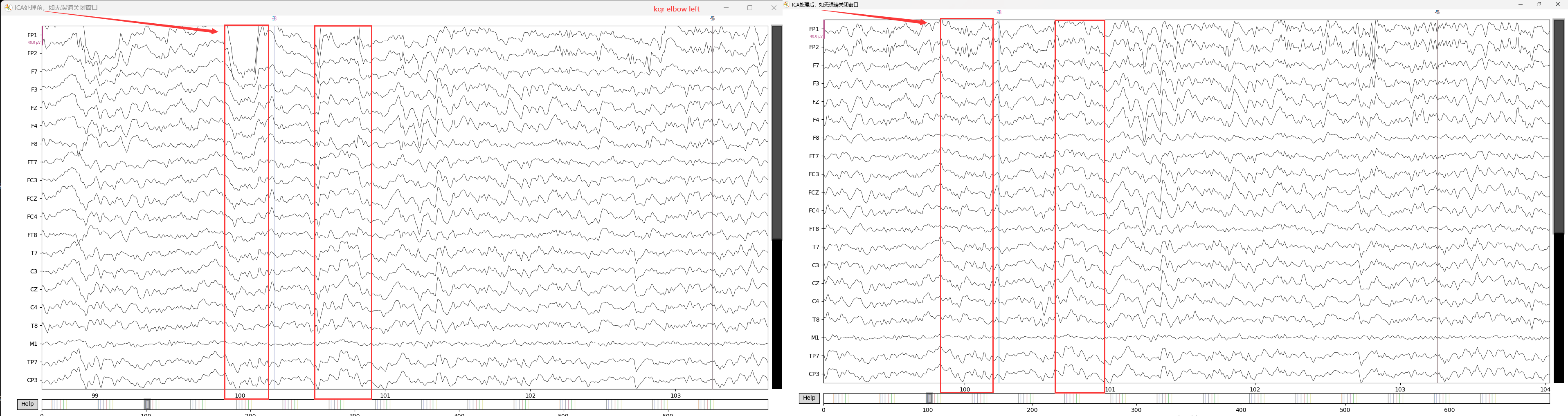
7.2 ICA成分剔除
1 | ''' 3. 查看选择去除的成分个数 ''' |
8. 通道定位 *
这一步一般不需要,只不过是因为我的电极重新布置了,所以得重新定位
自定义电极位置,需要自定义电极布局文件对数据进行通道定位可以查看这篇文章。
1 | # 查看通道名称 |
9. 保存预处理后的数据
1 | sub = 'sub1_' |
三、提取epoch,evoked *
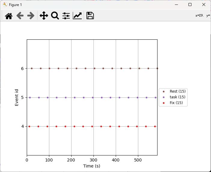
1. 绘制events图
1 | events, event_dict = mne.events_from_annotations(raw_ICA_rename) |
2. 根据marker提取epoch
1 | events = mne.events_from_annotations(raw_ICA_rename) |
3. 目视并手动去除伪迹依然严重的epoch
1 | task_epochs = epochs['task'] |
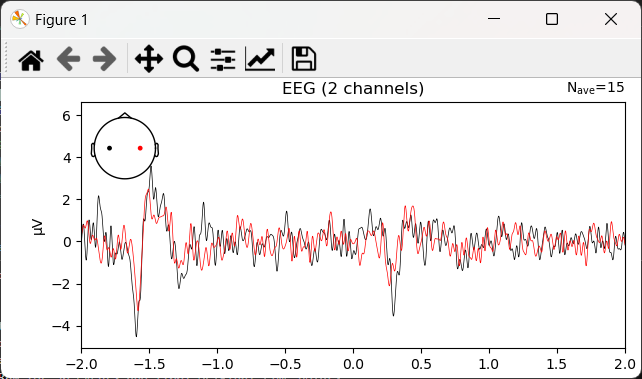
4. 绘制evoked时域波形
1 | task_evoked = task_epochs.average() |
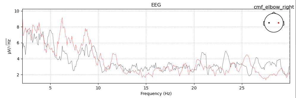
5. 绘制evoked的psd
1 | task_evoked.crop(0,12).plot_psd(fmin=2, fmax=30, |
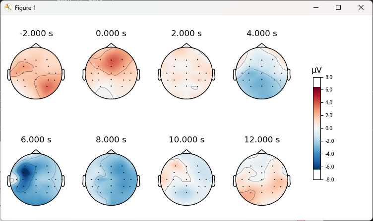
6. 绘制evoked某一时刻的脑地形图
1 | times = np.arange(-2, 14, 2) |
四. 绘制ERSP *
要计算ERSP,提取epoch时不需要基线矫正。
ERSP:反映了信号中不同频率的功率相对于特定时间点(例如信号出现)的变化程度。
事件相关同步化/去同步化:event-related synchronization / desynchronization (ERS/ERD)
- ERD 对应于特定频带内的功率相对于基线的降低。类似地,ERS 对应于功率的增加。
- ERDS 图是 ERD/ERS 在一定频率范围内的时间/频率表示形式。
- ERDS 地图也称为 ERSP(事件相关频谱扰动:event-related spectral perturbation, ERSP)。
参考:https://zh-1-peng.gitbook.io/eeg-analysis-note/ersp
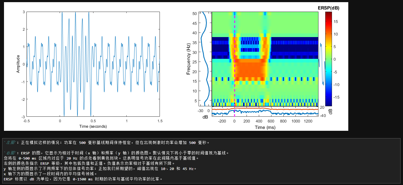
1. 定义小波函数计算时频谱
1 | from mne.time_frequency import tfr_morlet |
2. 绘制单通道ERSP
mode:‘mean’ | ‘ratio’ | ‘logratio’ | ‘percent’ | ‘zscore’ | ‘zlogratio’
Perform baseline correction by
-
subtracting the mean of baseline values (‘mean’)
-
dividing by the mean of baseline values (‘ratio’)
-
dividing by the mean of baseline values and taking the log (‘logratio’)
-
subtracting the mean of baseline values followed by dividing by the mean of baseline values (‘percent’)
-
subtracting the mean of baseline values and dividing by the standard deviation of baseline values (‘zscore’)
-
dividing by the mean of baseline values, taking the log, and dividing by the standard deviation of log baseline values (‘zlogratio’)
1 | def plotTF(taskPower, tmin1, tmax1, ch, fn): |
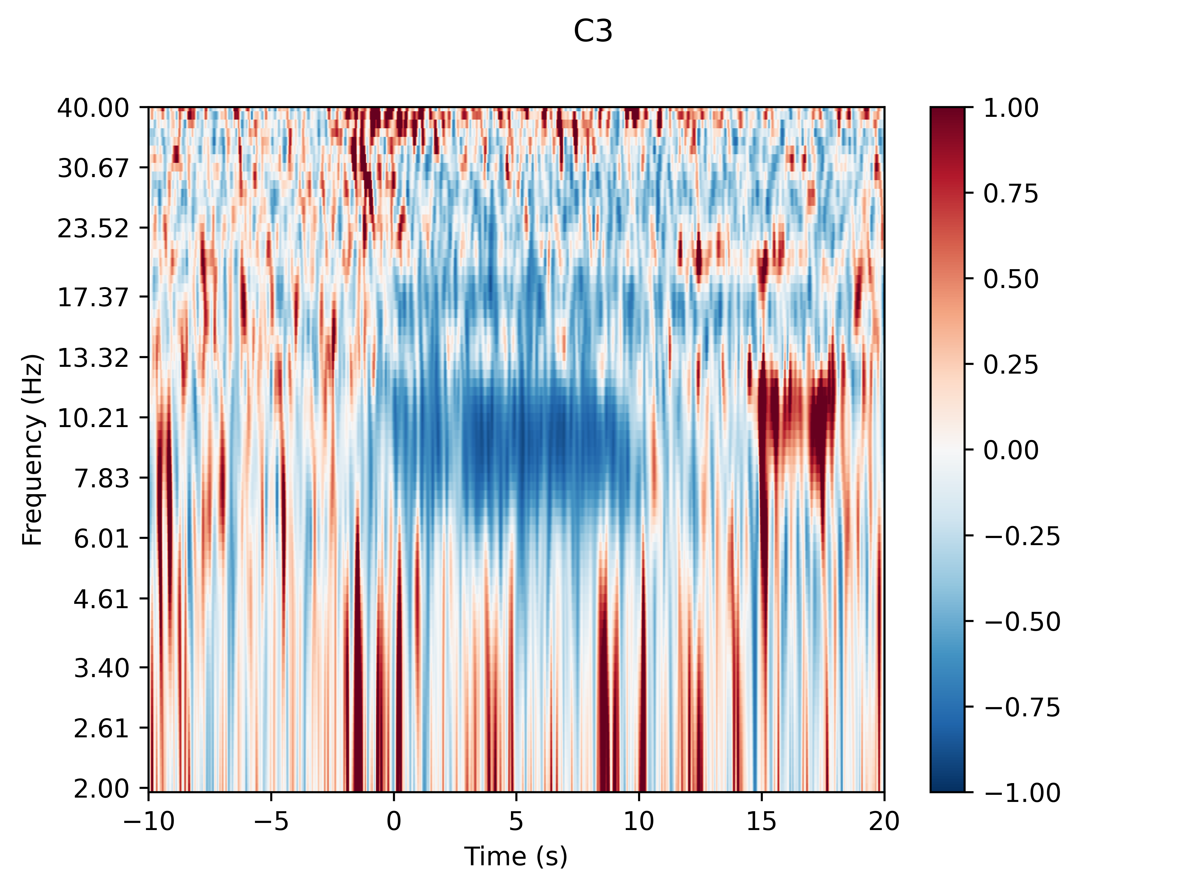
可以发现在任务时期,0~8s内,alpha频段的能量相较于基线明显下降,这是明显的ERD现象。
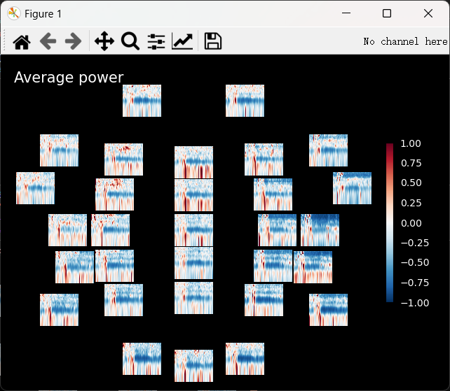
3. 绘制所有通道的ERSP
1 | task_power.plot_topo(baseline=(-7, -3), mode='percent', vmin=-1, vmax=1, title="Average power") # mode="logratio" |
4. 保存计算的时频谱
1 | import pickle |
5. 加载保存好的时频谱
1 | with open('task_power.pkl', 'rb') as f: |
6. 时间进程上特定频段power的变化
1 | def getPowerDataFrameTime(power_task, ch_pair): |
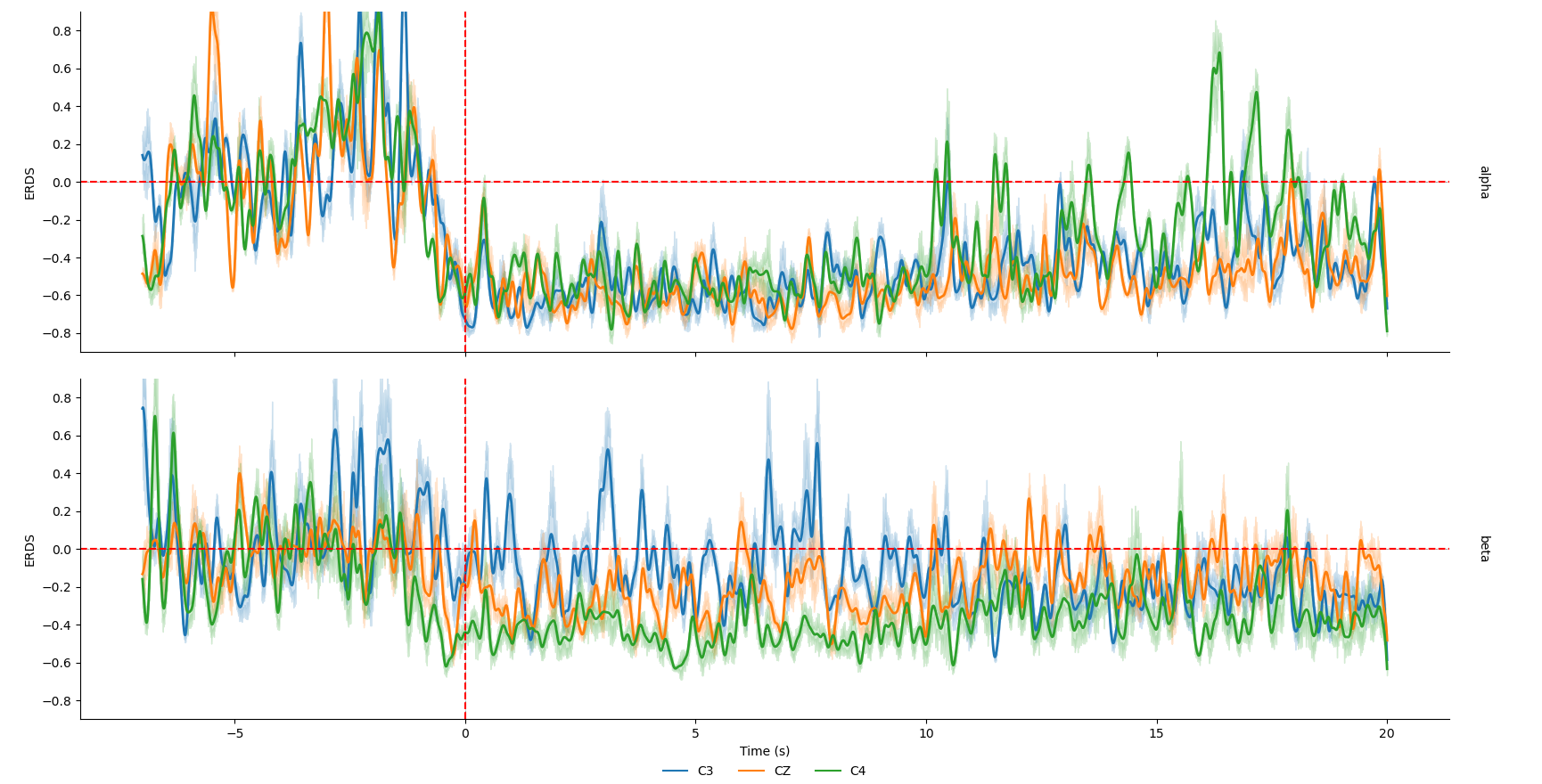
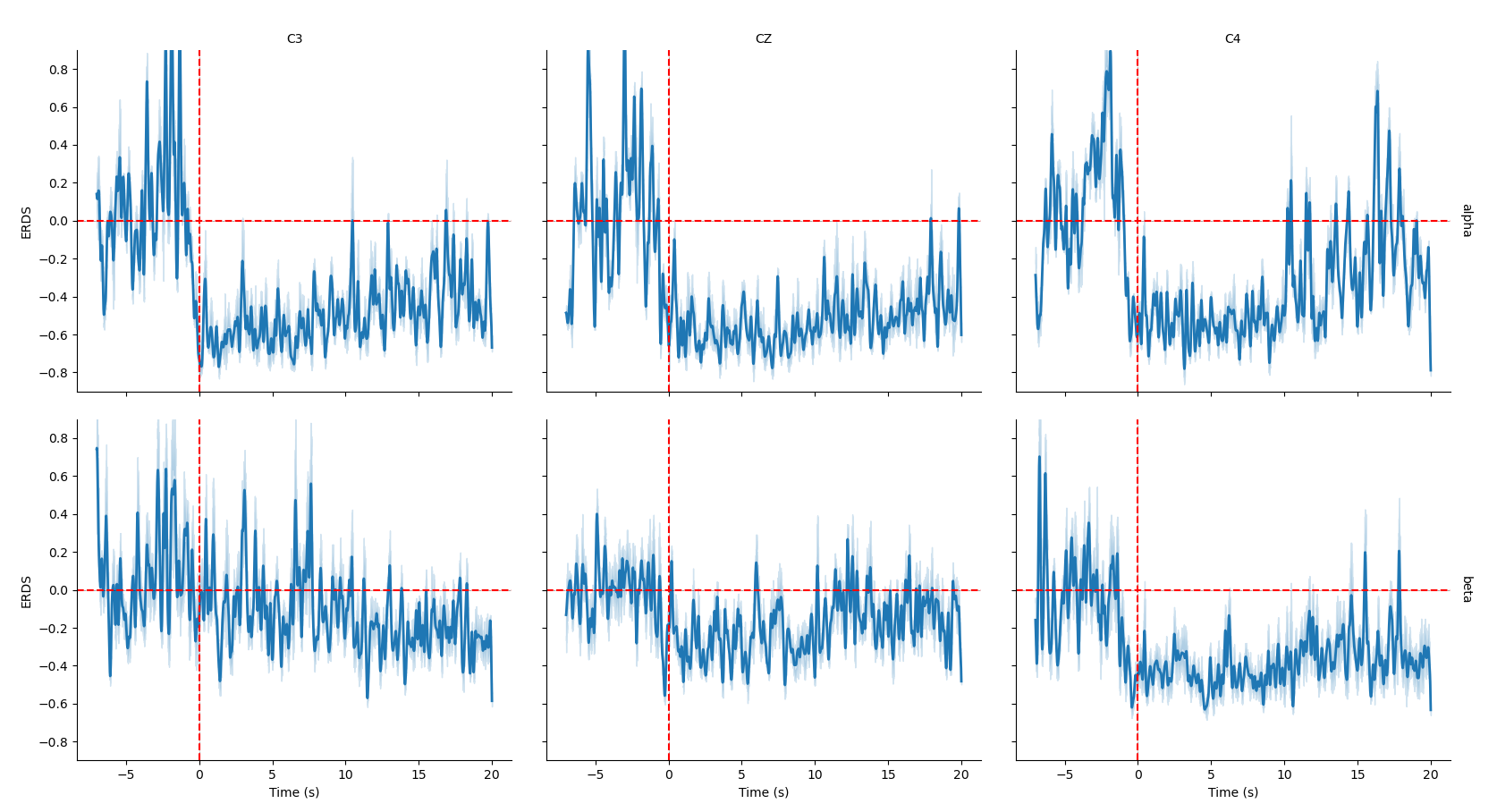
另一种画法
1 | g = sns.FacetGrid(task_power_time, row="band", col="channel", margin_titles=True) |
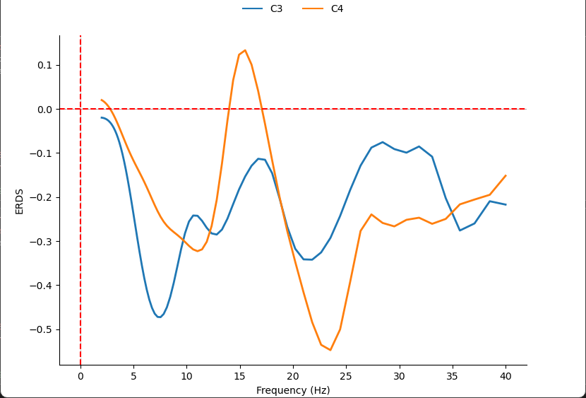
7. 频段进程上特定时间段power的变化
1 | def getPowerDataFrameBand(power_task, ch_pair): |
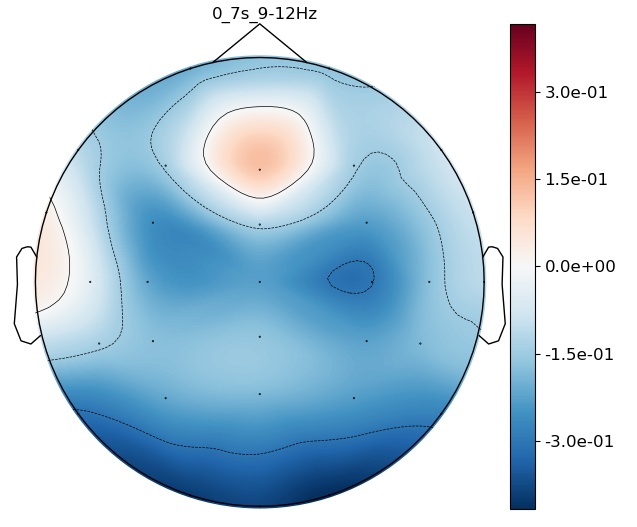
8. 绘制ERSD Map
可以选择频段和时间区间
1 | def plotTopoMap(taskPower, tmin1, tmax1, fn): |
以上就是从EEG预处理到绘制ERSP的全部过程,这里考虑了很多情况,步骤有点多,如果想要修改但不知道怎么改的可以给我留言哦。

